Conditional Formatting in Excel: Complete Guide with Examples & Tips

Excel becomes much easier to understand when important values can stand out without manually changing the formatting of every cell. Conditional Formatting in Excel does exactly that. It allows you to automatically change the appearance of cells when they meet a particular condition.

For example, you can highlight marks below 40 in red, show sales above ₹50,000 in green, identify duplicate names, display the highest values, or use color scales to understand a large set of numbers quickly. The formatting changes automatically whenever the underlying data changes.

For students, teachers, office employees, data-entry operators, and competitive-exam aspirants, this feature can save time and make Excel worksheets much easier to read. Instead of scanning hundreds of rows manually, you can let Excel visually identify the information you are looking for.

This guide explains Conditional Formatting in Excel from the basics to more advanced techniques, including rules, formulas, duplicate values, dates, entire-row highlighting, and common mistakes.

Visit More:-

What Is Conditional Formatting in Excel?

Conditional Formatting in Excel is a feature that automatically changes the visual formatting of a cell or range when its value meets a specified condition. You can use it to apply colors, icons, data bars, and other visual effects based on the data.

The important idea is simple:

Condition → Excel checks the cell → Matching cells receive formatting

For example, suppose you have the following student marks:

Student	Marks
Rahul	82
Neha	67
Aman	35
Priya	91
Rohit	28

You could create a conditional formatting rule such as:

Highlight cells less than 40 with red fill.

Excel would automatically highlight Aman’s and Rohit’s marks.

If you later change Rohit’s marks from 28 to 55, Excel can automatically remove the highlighting because the cell no longer satisfies the condition.

That automatic behavior is what makes conditional formatting so useful.

Why Is Conditional Formatting Important?

Conditional formatting helps you understand data visually instead of reading every value individually.

Imagine a worksheet containing 2,000 examination records. Finding every student who scored less than 40 manually would take time and could lead to mistakes. With a simple rule, Excel can identify those values instantly.

It is especially useful for:

Finding unusually high or low values
Highlighting failed or passed students
Identifying duplicate records
Tracking deadlines
Monitoring attendance
Comparing sales figures
Checking inventory levels
Identifying missing or problematic entries
Finding the top and bottom performers
Understanding trends in large datasets

The biggest benefit is that the formatting updates when the data changes. You do not need to repeatedly apply colors by hand.

How Does Conditional Formatting Work?

Conditional formatting works by applying a rule to one or more cells.

A rule contains two basic parts:

Condition: What should Excel check?

Format: What should Excel do when the condition is true?

For example:

If a student’s marks are below 40, fill the cell with red.

Here:

Condition = Marks < 40
Formatting = Red fill

Another example:

If sales are greater than ₹1,00,000, use green text.

Here:

Condition = Sales > 100000
Formatting = Green text

Excel can also evaluate formulas, text, dates, percentages, and relationships between different cells.

Where Is Conditional Formatting Located in Excel?

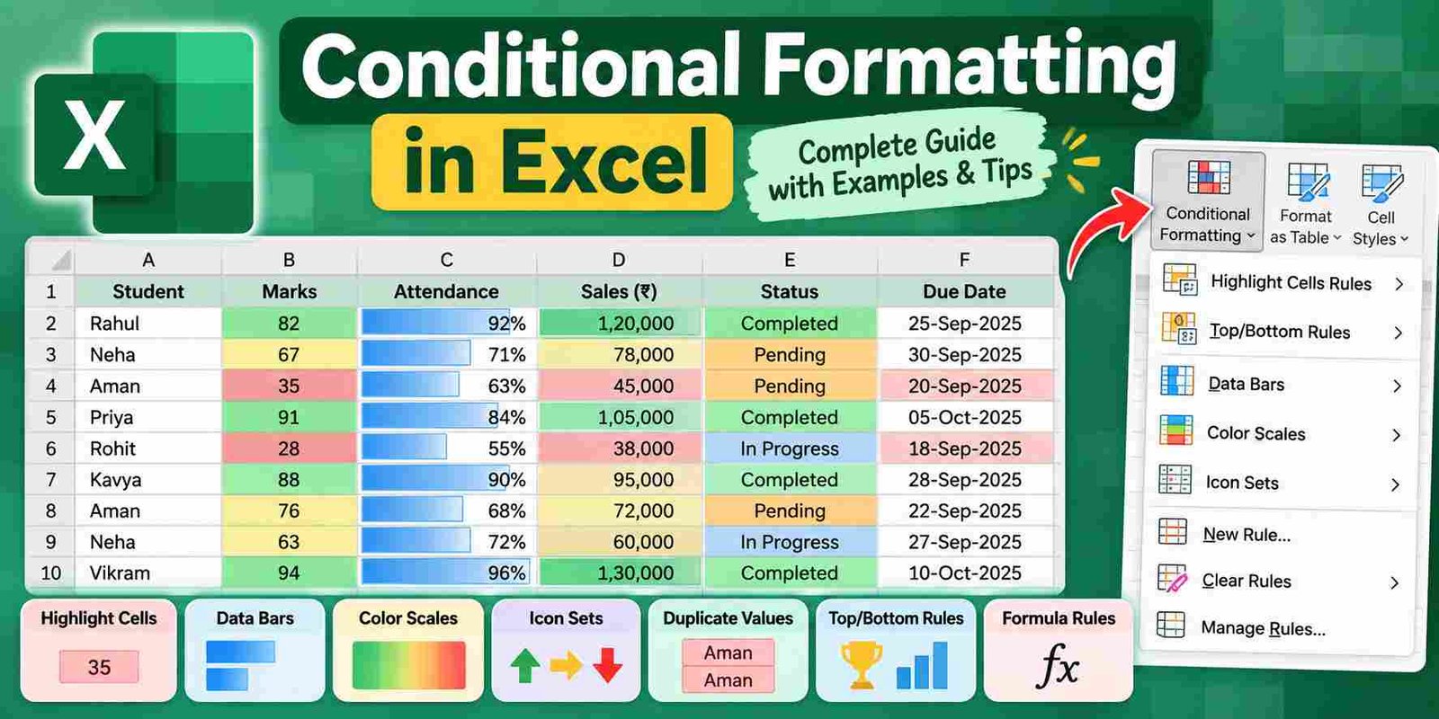
The Conditional Formatting option is available on the Home tab in the Excel ribbon.

To access it:

Open your Excel worksheet.
Select the cells you want to format.
Go to the Home tab.
Find the Styles section.
Click Conditional Formatting.

A dropdown menu will appear with several options.

Common options include:

Highlight Cells Rules
Top/Bottom Rules
Data Bars
Color Scales
Icon Sets
New Rule
Clear Rules
Manage Rules

The exact appearance may vary slightly between Excel versions, but the basic functionality remains similar.

Conditional Formatting in Excel guide with highlighted cells, data bars, color scales, and formatting rules — Conditional Formatting in Excel with examples of highlight rules, data bars, color scales, and icon sets

Main Types of Conditional Formatting in Excel

Excel provides several ways to create visual rules. Understanding these categories makes it much easier to choose the right option.

Type	Main Purpose
Highlight Cells Rules	Highlight values meeting a condition
Top/Bottom Rules	Identify highest or lowest values
Data Bars	Display values as horizontal bars
Color Scales	Compare values using colors
Icon Sets	Represent values with icons
Formula Rules	Create customized conditions
Duplicate Values	Find duplicate or unique entries

Let’s examine each one.

Highlight Cells Rules

Highlight Cells Rules are used when you want Excel to format cells based on simple comparisons such as greater than, less than, equal to, or containing particular text.

To use this feature:

Select the required range.
Go to Home → Conditional Formatting.
Select Highlight Cells Rules.
Choose a suitable rule.
Enter the required value.
Select a formatting style.
Click OK.

The available rules generally include options such as:

Greater Than
Less Than
Between
Equal To
Text That Contains
A Date Occurring
Duplicate Values

Greater Than

Suppose you have sales data:

Employee	Sales
A	45000
B	78000
C	120000
D	65000

To highlight sales above ₹70,000:

Select the sales column.
Open Conditional Formatting.
Choose Highlight Cells Rules → Greater Than.
Enter 70000.
Select the desired format.
Click OK.

Excel will automatically highlight values above 70,000.

Less Than

This is particularly useful for marks and performance data.

Suppose a passing mark is 40.

Select the marks and choose:

Conditional Formatting → Highlight Cells Rules → Less Than → 40

You can then choose red formatting.

Between

The Between rule is useful when you need to identify values within a range.

For example, you could highlight marks between 60 and 80.

This can be useful for analyzing:

Moderate scores
Age groups
Sales ranges
Price ranges
Attendance percentages

Equal To

Use this when a specific value needs to be identified.

For instance, you could highlight cells containing exactly 0.

This can help identify:

Zero sales
Zero attendance
Empty stock levels represented by 0
Zero marks in a particular subject

Text That Contains

Conditional formatting is not limited to numbers.

Suppose a column contains:

Status
Pending
Completed
Pending
Cancelled

You can highlight all cells containing the word Pending.

This can make task-management sheets easier to monitor.

How to Highlight Duplicate Values in Excel

Duplicate values are common in large datasets. Excel can identify them automatically.

For example, suppose a list of registration numbers contains repeated entries.

To find duplicates:

Select the relevant cells.
Go to Home → Conditional Formatting.
Select Highlight Cells Rules.
Click Duplicate Values.
Choose a formatting style.
Click OK.

Excel will visually mark repeated values.

This is useful when checking:

Student registration numbers
Employee IDs
Invoice numbers
Product codes
Customer names
Application numbers

You can also choose to highlight unique values instead of duplicates.

Top and Bottom Rules

Sometimes you do not want to compare values against a fixed number. Instead, you want Excel to identify the highest or lowest values within the selected range.

That is where Top/Bottom Rules are useful.

Common options include:

Top 10 Items
Top 10%
Bottom 10 Items
Bottom 10%
Above Average
Below Average

Top 10 Items

Suppose you have marks for 100 students and want to highlight the 10 highest marks.

Select the marks and choose:

Conditional Formatting → Top/Bottom Rules → Top 10 Items

Excel will highlight the highest ten values.

The number does not have to remain 10. You can enter another number when the rule dialog box appears.

Top 10 Percent

This works differently.

Instead of selecting a fixed number of values, Excel identifies the top percentage of values.

For example, if there are 100 students and you select the top 10%, Excel identifies the top 10 values.

Bottom 10 Items

This is useful for identifying the lowest-performing records.

In a marks sheet, it could help a teacher quickly identify students who may need additional academic support.

Above Average

Excel can automatically highlight values that are above the average of the selected range.

This can be useful for:

Comparing student marks
Evaluating monthly sales
Analyzing attendance
Reviewing expenses

Data Bars in Excel

Data Bars display a horizontal bar inside each cell based on the value of that cell.

For example:

Sales
20
50
80
100

The cell containing 20 receives a shorter bar, while the cell containing 100 receives a much longer bar.

To apply Data Bars:

Select the numerical range.
Go to Home → Conditional Formatting.
Select Data Bars.
Choose a style.

Data bars are useful because you can compare values visually without creating a separate chart.

For large tables, this can make patterns immediately visible.

Color Scales

Color Scales use different colors to represent low, medium, and high values in a selected range.

A common pattern is:

Lower values → one color
Middle values → another color
Higher values → a third color

For example, in a marks worksheet:

Student	Marks
A	32
B	54
C	68
D	82
E	94

A color scale can make it visually obvious which values are relatively low or high.

To apply one:

Select the range.
Go to Conditional Formatting.
Select Color Scales.
Choose an appropriate scale.

Color scales are particularly helpful when looking at a large matrix of numbers.

Icon Sets

Icon Sets add symbols to cells based on their values.

Depending on the selected icon set, Excel may display:

Arrows
Traffic lights
Flags
Ratings
Shapes
Other visual indicators

For example, arrows can represent whether values are relatively high, average, or low.

Icon Sets can be useful for dashboards and performance reports because they allow users to understand the data quickly.

However, icons should be used carefully. They can become confusing when the worksheet contains many different rules or when the meaning of each icon is unclear.

Using Custom Conditional Formatting Rules

The built-in options are useful, but sometimes you need a condition that Excel’s simple menus cannot express.

For those situations, use New Rule.

To create a custom rule:

Select the required range.
Go to Home → Conditional Formatting → New Rule.
Choose the type of rule.
Define the condition.
Select Format.
Choose the font, fill, border, or other formatting.
Click OK.

Custom rules are especially powerful when combined with formulas.

Formula-Based Conditional Formatting

Formula-based conditional formatting allows Excel to evaluate a formula and then apply formatting when that formula returns TRUE.

This is one of the most useful advanced features of conditional formatting.

For example, suppose:

Column A = Student Name
Column B = Marks

You want to highlight the student’s entire row when marks are below 40.

You could use a formula such as:

=$B2<40

The dollar sign is important because it controls how the reference behaves when Excel applies the rule across the selected range.

Why Is the Dollar Sign Used?

Consider the formula:

=$B2<40

Here:

$B keeps the column fixed.
2 is allowed to change by row.

So when Excel evaluates the next row, it checks B3, then B4, then B5, and so on.

This allows one rule to work across an entire table.

How to Highlight an Entire Row Based on a Cell Value

This is a very useful technique for student records, task lists, employee data, and financial worksheets.

Suppose your worksheet has:

Name	Marks	Status
Rahul	75	Pass
Aman	32	Fail
Priya	88	Pass

You want to highlight the whole row whenever the marks are below 40.

Steps:

Select the complete data range, for example A2:C100.
Open Conditional Formatting.
Select New Rule.
Choose Use a formula to determine which cells to format.
Enter:

=$B2<40

Click Format.
Choose a fill color.
Click OK.

Now the complete row will be formatted when the corresponding value in column B is below 40.

This method is much more powerful than simply highlighting the mark cell.

Conditional Formatting Based on Text

You can create rules based on text values as well.

Suppose your worksheet has a task status column:

Task	Status
Report	Completed
Data Entry	Pending
Review	In Progress

You can format rows based on the status.

For example, a formula such as:

=$C2="Pending"

can be used to identify pending tasks when column C contains the status.

Similarly:

=$C2="Completed"

can identify completed work.

This approach is useful for:

Student assignment tracking
Office task lists
Project management
Application status
Payment tracking
Inventory management

Conditional Formatting Based on Dates

Dates can also be used with conditional formatting.

For example, you may want to identify:

Today’s tasks
Upcoming deadlines
Overdue work
Recent dates
Older records

Suppose column D contains deadlines.

A formula can compare the date with today’s date.

For example:

=$D2<TODAY()

can be used to identify dates that have already passed, provided the cells contain valid Excel dates and the desired range is structured appropriately.

You could then apply a noticeable format to overdue entries.

This is particularly useful for:

Assignment deadlines
Exam schedules
Application deadlines
Bill due dates
Project milestones
Subscription renewals

Conditional Formatting for Attendance

Students and teachers can use conditional formatting to monitor attendance.

Suppose a worksheet contains attendance percentages.

Student	Attendance
Rahul	92%
Aman	71%
Priya	84%
Neha	63%

You can create rules to visually distinguish lower and higher attendance.

For example:

Below a chosen threshold → warning formatting
Above a chosen threshold → positive formatting

The exact attendance requirement can depend on the school, college, university, or institution, so the spreadsheet rule should be based on the applicable requirement rather than assuming one universal percentage.

Conditional Formatting for Student Marks

This is one of the easiest ways for students and teachers to learn the feature.

Suppose marks are in cells B2:B50.

You could create rules such as:

Condition	Example Formatting
Less than 40	Highlight
40 to 59	Another format
60 to 79	Another format
80 and above	Another format

This creates a quick visual classification of performance.

You can also use:

Data bars to compare marks
Color scales to see overall performance
Top 10 rules to identify highest marks
Below Average to identify lower-performing scores
Duplicate rules to detect repeated values

Conditional Formatting for Exam Preparation

Competitive-exam aspirants can also use this feature while preparing study schedules.

Imagine an Excel sheet containing:

Subject	Questions Attempted	Accuracy
Reasoning	120	85%
Quantitative Aptitude	100	68%
English	150	91%

Conditional formatting can highlight accuracy percentages that fall below your personal target.

For example, if you decide that anything below 75% needs additional practice, you can create a rule based on that value.

This does not replace analysis, but it helps you identify where to spend more time.

Conditional Formatting for Sales Data

In an office environment, conditional formatting can help employees understand sales data quickly.

Suppose monthly sales are recorded for different employees.

You might want to:

Highlight sales above a target
Identify values below a minimum threshold
Display top-performing employees
Use data bars to compare sales
Use color scales for a quick overview

Instead of manually coloring every record, Excel handles the visual formatting automatically.

Conditional Formatting for Inventory

Inventory spreadsheets often contain hundreds or thousands of products.

Suppose a table contains:

Product	Stock
Pen	125
Notebook	42
Folder	8
Marker	3

A low-stock rule can make products requiring attention immediately visible.

For example, you could create a rule that highlights quantities below a chosen minimum level.

This is useful because the same rule continues to work when stock quantities are updated.

Multiple Conditional Formatting Rules

A worksheet can contain more than one rule.

For example, a marks column could have:

Less than 40 → one format
40 to 59 → another format
60 to 79 → another format
80 or more → another format

Another column could simultaneously use:

Duplicate-value highlighting
Data bars
Top-value rules

However, using too many rules can make a worksheet visually confusing.

Good spreadsheet design is not about adding the maximum number of colors. It is about making important information easier to understand.

How to Manage Conditional Formatting Rules

When several rules exist, Manage Rules becomes important.

Go to:

Home → Conditional Formatting → Manage Rules

Here you can see the rules applied to the worksheet.

Depending on the Excel version and rule type, you may be able to:

Edit a rule
Delete a rule
Change the order
Modify the range
Review which cells the rule applies to

This is particularly helpful when conditional formatting does not appear to work as expected.

Understanding Rule Priority

When multiple rules apply to the same cells, their order can affect the result.

For example, imagine two rules:

Highlight values below 40 with one format.
Highlight values below 60 with another format.

A value of 30 satisfies both conditions.

Excel therefore needs to determine how the rules interact. Rule order and settings in the rule manager become important in situations like this.

When troubleshooting conditional formatting, always check the rules applied to the range instead of creating another rule immediately.

How to Remove Conditional Formatting

There are several ways to remove it.

To clear rules from selected cells:

Select the cells.
Go to Home → Conditional Formatting.
Select Clear Rules.
Choose the appropriate option.

Depending on your selection, you can clear rules from:

Selected cells
Entire worksheet
Other applicable ranges

Be careful when clearing rules because it can remove formatting from more cells than intended.

Conditional Formatting vs Manual Formatting

Manual formatting means you select cells and apply formatting yourself.

For example:

Select a cell
Click Fill Color
Choose red
Repeat for another cell

Conditional formatting works differently.

You define the condition once, and Excel determines which cells should receive the formatting.

Manual Formatting	Conditional Formatting
Applied manually	Applied automatically
May need repeated changes	Updates with data
Useful for fixed design	Useful for changing conditions
Can take more time for large datasets	Efficient for large datasets

For dynamic data, conditional formatting is usually more convenient because the visual result can change automatically.

Conditional Formatting vs Filters

These two features are often confused.

Filtering changes which rows are displayed.

Conditional formatting changes how cells look.

For example, suppose you have 500 student records.

A filter can show only students with marks below 40.

Conditional formatting can keep all 500 records visible while highlighting the low marks.

You can also use both features together.

Common Mistakes in Conditional Formatting

Even though the feature is easy to start with, several mistakes can produce unexpected results.

Selecting the Wrong Range

If you select only part of the table, the rule will not affect the rest of the data.

Always check the range before creating a rule.

Using the Wrong Cell Reference

Formula rules are particularly sensitive to cell references.

For example:

=$B2<40

and

=B2<40

may behave differently when applied across multiple columns, because absolute and relative references control how the formula changes.

Using Text Instead of Numbers

If numeric values have been stored as text, numerical conditions may not behave as expected.

For example, a cell containing "50" as text is not necessarily handled the same way as a true numeric 50 in every calculation or rule scenario.

Applying Too Many Rules

A worksheet covered in different colors and icons can become difficult to read.

Use conditional formatting to emphasize meaningful information rather than every possible difference.

Forgetting to Check Rule Priority

When several rules overlap, inspect Manage Rules.

The problem may not be the formula itself. The issue could be how multiple rules interact.

How to Make Conditional Formatting More Effective

A few simple practices can improve your worksheets significantly.

Use Meaningful Formatting

Choose formatting that communicates a clear message.

For example, a warning color for overdue work makes sense because the visual distinction has a purpose.

Keep Colors Consistent

If red means “attention required” in one part of a workbook, using red for completely unrelated information elsewhere may confuse the reader.

Avoid Excessive Decoration

Conditional formatting should improve understanding.

If every cell has a different color, the important values become harder to notice.

Test Rules With Different Values

After creating a rule, change a few values temporarily and see whether the formatting changes as expected.

This is particularly useful when working with formula-based rules.

Use Clear Labels

If icons or colors are used in a report, the meaning should be understandable from the surrounding headers or notes.

Important Keyboard Shortcuts and Navigation Tips

Conditional formatting does not depend on a single keyboard shortcut, but efficient Excel navigation can make the process faster.

For students learning Excel, remember the basic path:

Home → Conditional Formatting

You can also use familiar Excel keyboard navigation to select ranges before creating the rule.

The bigger time-saving technique is not memorizing a shortcut. It is understanding exactly what condition you want to test before opening the Conditional Formatting menu.

Advanced Example: Highlight Duplicate Student Names

Suppose the student names are stored in A2:A100.

To highlight duplicates:

Select A2:A100.
Open Conditional Formatting.
Choose Highlight Cells Rules.
Select Duplicate Values.
Choose a formatting style.
Click OK.

Excel identifies names that appear more than once.

However, remember that duplicate names do not necessarily mean duplicate students. Two different students can have the same name.

For more reliable duplicate checking, use a unique identifier such as registration number or student ID when available.

Advanced Example: Highlight Rows With “Pending” Status

Suppose:

Column A = Application Number
Column B = Candidate Name
Column C = Status

You want the complete row highlighted whenever status is “Pending.”

Select the full table and create a formula-based rule:

=$C2="Pending"

Then choose the desired formatting.

This technique is useful for tracking:

Applications
Payments
Documents
Approvals
Tasks
Complaints
Orders

Advanced Example: Highlight the Highest Value

Suppose monthly expenses are recorded in B2:B20.

You can use a Top/Bottom rule to highlight the highest value.

Alternatively, a formula can compare a cell against the maximum value of the range.

For example:

=B2=MAX($B$2:$B$20)

This can be useful when you need more control over the formatting logic.

The range inside MAX remains fixed because of the dollar signs.

Advanced Example: Highlight Cells Based on Another Column

One of the most practical uses of formula-based conditional formatting is checking one column while formatting another.

Suppose:

Task	Due Date	Status
Assignment	25 Sep	Pending
Project	30 Sep	Completed
Revision	27 Sep	Pending

You may want to highlight rows based on status rather than the text itself.

A formula such as:

=$C2="Pending"

can be applied to the whole table.

This demonstrates an important idea:

The cell being checked does not always have to be the cell receiving the formatting.

Important Points About Relative and Absolute References

Understanding cell references is essential for advanced conditional formatting.

There are three common forms:

A1

Both column and row can change.

$A$1

Both column and row remain fixed.

$A1

Column stays fixed, while the row can change.

A$1

Row stays fixed, while the column can change.

When creating a conditional formatting formula, ask:

Which part should remain fixed, and which part should change?

For an entire-row rule where column B contains the condition, $B2 is often useful because the condition always comes from column B while the row number changes.

Benefits of Conditional Formatting in Excel

Conditional formatting offers several practical advantages.

Saves Time

Once the rule is created, Excel performs the formatting automatically.

Makes Data Easier to Understand

Colors, bars, and icons can make patterns visible quickly.

Reduces Manual Work

You do not need to repeatedly identify and color matching values.

Helps Find Errors

Duplicate entries, unusual values, and missing information can become easier to spot.

Supports Better Data Analysis

Visual patterns often become clearer when values are formatted dynamically.

Works Well With Changing Data

When values change, the formatting can update automatically according to the rules.

Limitations of Conditional Formatting

Conditional formatting is powerful, but it is not a replacement for every Excel feature.

It has some practical limitations.

Too Much Formatting Can Reduce Readability

Excessive colors and icons can create visual clutter.

Complex Rules Can Be Difficult to Maintain

A workbook with many formulas and overlapping rules may be harder for another person to understand.

Incorrect References Can Produce Wrong Results

Formula-based conditional formatting requires careful cell referencing.

Formatting Is Not the Same as Analysis

A highlighted cell tells you that a condition is met. It does not automatically explain why the value changed or what action should be taken.

For deeper analysis, you may still need formulas, PivotTables, charts, filters, or other Excel features.

Practical Excel Learning Exercise

A good way to learn conditional formatting is to practice with a small worksheet.

Create this table:

Student	Maths	Reasoning	English
Rahul	82	75	68
Aman	35	52	44
Neha	91	87	94
Priya	63	71	80
Rohit	28	40	33

Now practice the following:

Highlight marks below 40.
Highlight marks above 80.
Apply a color scale.
Add data bars.
Identify the top values.
Highlight duplicate values after creating a few duplicates.
Create a rule that highlights an entire row when Maths marks are below 40.

This exercise covers both beginner and advanced concepts.

Conditional Formatting for Competitive Exams

Excel is frequently included in basic computer-awareness and office-skills learning. Conditional formatting can therefore be worth understanding for students preparing for computer-related questions.

Important concepts to remember include:

Conditional formatting changes cell appearance based on rules.
Rules can be based on numbers, text, dates, or formulas.
Highlight Cells Rules are useful for simple comparisons.
Top/Bottom Rules identify high and low values.
Data Bars represent values visually.
Color Scales compare values through color intensity.
Icon Sets provide visual indicators.
Custom formulas allow advanced conditions.
Manage Rules is useful for editing and troubleshooting.
Conditional formatting is different from filtering.

A Simple Memory Trick

Remember the main purpose as:

“Condition decides the Format.”

Whenever a question asks about automatically formatting cells depending on their values, think of Conditional Formatting.

Important Points to Remember

Before using the feature in a real workbook, keep these points in mind:

Select the correct range before creating the rule.
Decide the condition clearly.
Choose formatting that has a purpose.
Use formulas when built-in rules are not enough.
Understand absolute and relative references.
Check Manage Rules when multiple conditions overlap.
Avoid unnecessary colors.
Test the rule by changing sample values.
Use identifiers rather than names alone when checking duplicates.
Remember that conditional formatting changes appearance; it does not change the underlying data.

Frequently Asked Questions

What is Conditional Formatting in Excel?

Conditional Formatting in Excel is a feature that automatically applies formatting to cells when they meet a specified condition. The condition can be based on numbers, text, dates, formulas, or other criteria.

How do I apply Conditional Formatting in Excel?

Select the cells, go to Home → Conditional Formatting, choose a rule such as Greater Than or Duplicate Values, define the condition, select the formatting, and click OK.

Can Conditional Formatting in Excel be based on a formula?

Yes. You can create a new rule using Use a formula to determine which cells to format. Formula-based rules are useful when the condition is more complex than the built-in options.

Can I highlight an entire row using Conditional Formatting?

Yes. Select the full table and use a formula that checks the relevant column. For example, =$B2<40 can highlight rows based on the value in column B when the rule is applied to the appropriate range.

How can I find duplicate values in Excel?

Select the required range and choose Home → Conditional Formatting → Highlight Cells Rules → Duplicate Values. Excel will then visually identify repeated entries.

Can Conditional Formatting work with dates?

Yes. Excel can apply formatting based on dates, including rules for dates occurring within certain periods. Formula-based rules can also be used for more customized date conditions.

What is the difference between Conditional Formatting and normal formatting?

Normal formatting is applied manually and generally remains until you change it. Conditional formatting is controlled by a rule, so Excel can automatically apply or remove the formatting as the data changes.

Can I use multiple Conditional Formatting rules on the same cells?

Yes. Multiple rules can be applied to overlapping or different ranges. When rules overlap, their priority and interaction should be checked using Manage Rules.

Why is my Conditional Formatting not working?

Common reasons include an incorrect selected range, an incorrect formula reference, values stored as text instead of numbers, conflicting rules, or an unexpected rule order. Checking Manage Rules is a useful troubleshooting step.

Can Conditional Formatting change the actual cell value?

No. Conditional formatting normally changes the visual appearance of a cell, such as its fill, font, border, data bar, or icon. It does not itself change the underlying value.

Is Conditional Formatting useful for students?

Yes. Students can use it to track marks, attendance, study targets, mock-test performance, deadlines, and other academic data. It can make patterns easier to identify in a spreadsheet.

Which is better for large datasets: Color Scales or Data Bars?

Neither is universally better. Color scales are useful when comparing relative values across a range, while data bars provide a visual sense of the size of individual values. The better choice depends on what you want the worksheet to communicate.

Conclusion

Conditional Formatting in Excel is one of the most useful tools for making spreadsheet data easier to read, compare, and monitor. It starts with simple rules such as highlighting values greater than or less than a number, but it can also handle duplicates, dates, top and bottom values, data bars, color scales, icon sets, and custom formulas.

For beginners, the best way to learn is to start with simple examples such as student marks or attendance. Once those rules become familiar, move on to formula-based formatting and entire-row highlighting.

The most important concept is straightforward: define a condition, choose the formatting, and let Excel apply it automatically. With regular practice, Conditional Formatting in Excel can become a natural part of creating organized and useful worksheets.