
Excel becomes much more useful when you know how to find information quickly. Instead of manually checking rows and columns, you can use lookup functions to search a table and return the value you need. Two of the most useful functions for this purpose are VLOOKUP and XLOOKUP.
For example, imagine you have a student marks sheet containing roll numbers, names, classes, and marks. You know a student’s roll number, but you want Excel to automatically show that student’s name or marks. A lookup formula can do this in just a few seconds.
This guide explains How to use VLOOKUP and XLOOKUP in Excel step by step, starting with the basic idea and gradually moving toward practical examples, common mistakes, approximate matches, error handling, and real-world uses. The explanations are written for beginners, but the examples also cover concepts that are useful for office work, data analysis, competitive-exam preparation, and everyday spreadsheet tasks.
Visit More:-
- MS Word Tutorial
- MS Excel Tutorial
- MS PowerPoint Tutorial
- MS Paint Tutorial
- IF AND OR LOGICAL Functions in Excel Explained: Easy Guide
- How to Create and Use Pivot Tables in Excel for Beginners
- Most Useful Excel Keyboard Shortcuts to Save Time: Complete Guide
What Are VLOOKUP and XLOOKUP in Excel?
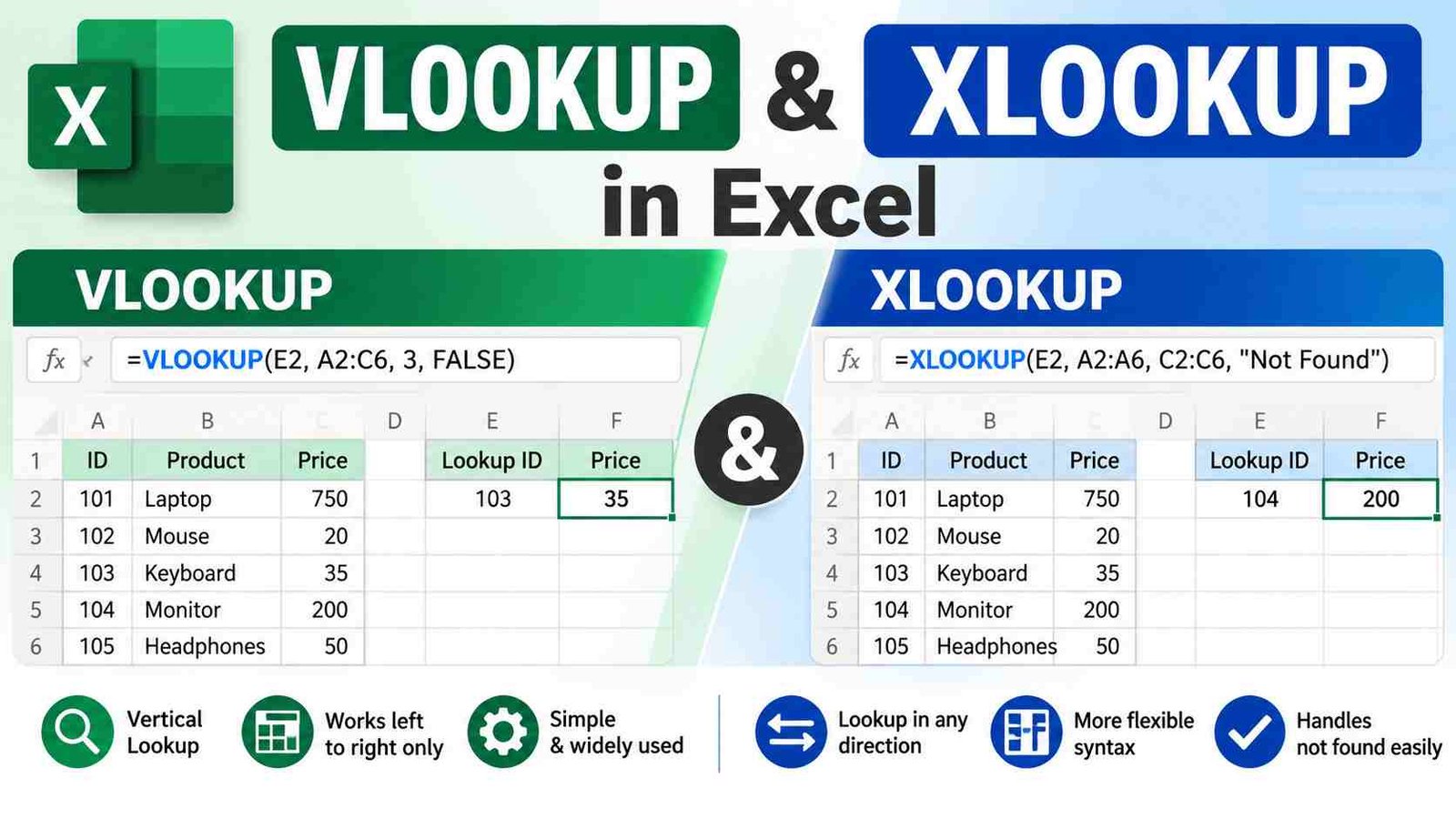
VLOOKUP and XLOOKUP are Excel lookup functions used to search for a value in a table and return related information from another column or range.
VLOOKUP has been used in Excel for many years and is still common in offices, older workbooks, and exam questions. XLOOKUP is a newer and more flexible lookup function available in newer versions of Excel.
The basic purpose of both functions is similar:
Find something in a data set and return the information associated with it.
For example, consider this table:
| Roll No. | Student Name | Class | Marks |
|---|---|---|---|
| 101 | Rahul | 10 | 82 |
| 102 | Neha | 10 | 91 |
| 103 | Aman | 10 | 76 |
| 104 | Priya | 10 | 88 |
Suppose cell F2 contains 103. You want Excel to display Aman automatically.
A lookup formula can search for 103 in the Roll No. column and return Aman from the Student Name column.
That is the central idea behind lookup functions.
Why Are Lookup Functions Important in Excel?
Lookup functions save time and reduce manual work. They are especially helpful when a worksheet contains hundreds or thousands of rows.
Imagine a salary sheet with 5,000 employees. Searching for a particular employee manually every time would be slow and frustrating. A lookup formula can find the employee ID and return the name, department, salary, joining date, or other related information almost instantly.
Some common uses include:
- Finding a student’s marks using a roll number
- Finding an employee’s salary using an employee ID
- Finding a product price using a product code
- Finding a department using an employee number
- Matching examination results with candidate IDs
- Retrieving customer information
- Checking inventory details
- Comparing two data tables
- Creating automated reports
- Preparing attendance and performance sheets
For students learning Excel, VLOOKUP is also useful because it teaches an important spreadsheet concept: using one piece of information to retrieve another piece of information from a structured data table.
Understanding VLOOKUP Before Using It
VLOOKUP stands for Vertical Lookup.
It searches for a value in the first column of a selected table and returns a corresponding value from another column in the same row.
The basic syntax is:
=VLOOKUP(lookup_value, table_array, col_index_num, [range_lookup])
Each argument has a specific purpose.
| Argument | Meaning |
|---|---|
| lookup_value | The value you want Excel to search for |
| table_array | The range containing the lookup table |
| col_index_num | The column number from which the result should be returned |
| range_lookup | Determines exact or approximate matching |
The syntax may initially look complicated, but it becomes easy when you break it into parts.
Suppose your table is in cells A2:D5 and you want to find the name for roll number 103:
=VLOOKUP(103,A2:D5,2,FALSE)
Here:
103is the value being searched.A2:D5is the table.2tells Excel to return the value from the second column of the table.FALSEtells Excel to find an exact match.
How to Use VLOOKUP in Excel Step by Step
Let’s learn VLOOKUP with a simple example.
Suppose your worksheet contains:
| A | B | C | D |
|---|---|---|---|
| Roll No. | Student Name | Class | Marks |
| 101 | Rahul | 10 | 82 |
| 102 | Neha | 10 | 91 |
| 103 | Aman | 10 | 76 |
| 104 | Priya | 10 | 88 |
Now suppose cell F2 contains the roll number 103, and you want the student’s name to appear in G2.
Step 1: Select the Result Cell
Click the cell where you want the answer to appear.
For this example, click G2.
Step 2: Start the VLOOKUP Formula
Type:
=VLOOKUP(
Excel will expect you to enter the lookup arguments.
Step 3: Enter the Lookup Value
The lookup value is the value you want to search for.
Since the roll number is in F2, type:
=VLOOKUP(F2,
Step 4: Select the Table
Select the complete table that contains the roll number and the information you want to return.
For example:
=VLOOKUP(F2,A2:D5,
The important point is that the lookup column must be the first column of the selected table.
Step 5: Enter the Column Number
The Student Name column is the second column within A2:D5.
Therefore, enter:
=VLOOKUP(F2,A2:D5,2,
Remember that VLOOKUP counts columns from the beginning of the selected range, not from the entire worksheet.
Step 6: Choose Exact Match
For roll numbers, employee IDs, product codes, and similar values, you normally want an exact match.
Enter:
FALSE
The completed formula is:
=VLOOKUP(F2,A2:D5,2,FALSE)
Press Enter.
Excel should return:
Aman
This is the basic VLOOKUP process.
Why Is FALSE Commonly Used in VLOOKUP?
The last argument of VLOOKUP controls the type of match.
FALSE means Excel should look for an exact match.
TRUE means Excel can return an approximate match.
For most beginner lookup tasks, exact matching is easier to understand and safer when searching for unique identifiers.
For example:
=VLOOKUP(F2,A2:D5,2,FALSE)
means:
Find exactly the value in F2 in the first column of A2:D5 and return the value from column 2.
You can also use 0 instead of FALSE for exact matching:
=VLOOKUP(F2,A2:D5,2,0)
Both represent an exact-match lookup.
VLOOKUP With Cell References
Using a cell reference is more useful than typing the lookup value directly into the formula.
For example:
=VLOOKUP(F2,A2:D5,2,FALSE)
If you change F2 from 103 to 104, the result changes automatically from Aman to Priya.
This makes your spreadsheet interactive.
You can create a simple search box where a user enters a roll number and Excel automatically displays the student’s name and marks.
For example:
=VLOOKUP(F2,A2:D5,2,FALSE)
for the name, and:
=VLOOKUP(F2,A2:D5,4,FALSE)
for the marks.
VLOOKUP Column Number Explained With an Easy Trick
One of the most common beginner mistakes is misunderstanding the column index.
Suppose you use:
A2:D5
The columns inside this table are counted like this:
| Column | VLOOKUP Number |
|---|---|
| A | 1 |
| B | 2 |
| C | 3 |
| D | 4 |
So:
=VLOOKUP(F2,A2:D5,2,FALSE)
returns the value from column B.
And:
=VLOOKUP(F2,A2:D5,4,FALSE)
returns the value from column D.
The numbering starts from 1 at the first column of the selected table.
VLOOKUP Approximate Match
VLOOKUP can also be used for approximate matches. This is useful for ranges or categories rather than unique IDs.
For example:
| Minimum Marks | Grade |
|---|---|
| 0 | F |
| 40 | D |
| 50 | C |
| 60 | B |
| 75 | A |
Suppose a student’s marks are in F2.
You could use:
=VLOOKUP(F2,A2:B6,2,TRUE)
If F2 contains 68, Excel can return B based on the highest matching minimum value.
Approximate matching is useful for things such as:
- Grade ranges
- Tax brackets
- Commission slabs
- Discount ranges
- Performance categories
- Score classifications
However, the lookup table needs to be properly arranged for approximate matching to work correctly.
Common VLOOKUP Errors and How to Fix Them
Beginners often see errors after writing a VLOOKUP formula. Most problems are caused by a small issue in the formula or data.
#N/A Error
#N/A usually means Excel could not find the lookup value.
For example:
=VLOOKUP(F2,A2:D5,2,FALSE)
If F2 contains 999 and 999 does not exist in the first column, Excel may return #N/A.
Check whether:
- The value actually exists.
- There are extra spaces.
- One value is stored as text and the other as a number.
- The lookup column is correct.
#REF! Error
This can happen when the column index is larger than the number of columns in the selected table.
For example:
=VLOOKUP(F2,A2:D5,6,FALSE)
The selected table contains only four columns, so column 6 does not exist within that range.
#VALUE! Error
This may occur because an argument in the formula is invalid or a value is being used incorrectly.
Check the formula carefully and ensure that each argument is valid.
Wrong Result
A wrong result can occur when approximate matching is used accidentally.
For exact lookups, use:
FALSE
or:
0
What Is XLOOKUP in Excel?
XLOOKUP is a newer Excel lookup function designed to make searching and returning data easier and more flexible.
Unlike VLOOKUP, XLOOKUP does not require you to specify a column number. Instead, you tell Excel exactly where to search and exactly where to return the result.
The basic syntax is:
=XLOOKUP(lookup_value, lookup_array, return_array, [if_not_found], [match_mode], [search_mode])
The most important three parts are:
- What are you looking for?
- Where should Excel look?
- What range should Excel return the result from?
For example:
=XLOOKUP(F2,A2:A5,B2:B5)
This means:
Find the value in F2 in A2:A5 and return the corresponding value from B2:B5.
If F2 contains 103, the result is Aman.
How to Use XLOOKUP in Excel Step by Step
Let’s use the same student table.
| Roll No. | Student Name | Class | Marks |
|---|---|---|---|
| 101 | Rahul | 10 | 82 |
| 102 | Neha | 10 | 91 |
| 103 | Aman | 10 | 76 |
| 104 | Priya | 10 | 88 |
Suppose F2 contains 103.
You want G2 to display the student’s name.
Step 1: Select the Result Cell
Click G2.
Step 2: Type XLOOKUP
Enter:
=XLOOKUP(
Step 3: Enter the Lookup Value
Use F2:
=XLOOKUP(F2,
Step 4: Select the Lookup Array
The Roll No. values are in A2:A5.
So enter:
=XLOOKUP(F2,A2:A5,
Step 5: Select the Return Array
The Student Name values are in B2:B5.
So the formula becomes:
=XLOOKUP(F2,A2:A5,B2:B5)
Press Enter.
Excel returns:
Aman
Notice that there is no column number.
That is one of the main differences between XLOOKUP and VLOOKUP.
XLOOKUP With a Custom Not-Found Message
One very useful feature of XLOOKUP is that you can specify what should appear when a match is not found.
For example:
=XLOOKUP(F2,A2:A5,B2:B5,"Student Not Found")
If F2 contains a roll number that does not exist, Excel will display:
Student Not Found
This can make reports easier for people to understand.
Instead of seeing:
#N/A
the worksheet can show a clear message.
How XLOOKUP Can Return Marks
Suppose you want marks instead of the student name.
The Marks column is D2:D5.
Use:
=XLOOKUP(F2,A2:A5,D2:D5)
For roll number 103, the result is:
76
This formula is easy to read because the lookup and return ranges are clearly visible.
XLOOKUP Can Search From Right to Left
One of the major advantages of XLOOKUP is that the return range does not need to be located to the right of the lookup range.
Consider this table:
| Student Name | Roll No. | Class | Marks |
|---|---|---|---|
| Rahul | 101 | 10 | 82 |
| Neha | 102 | 10 | 91 |
| Aman | 103 | 10 | 76 |
| Priya | 104 | 10 | 88 |
Suppose you want to search for Roll No. 103 and return the Student Name.
With XLOOKUP:
=XLOOKUP(F2,B2:B5,A2:A5)
This works because XLOOKUP allows the return range to be on either side of the lookup range.
Traditional VLOOKUP is more limited because its lookup column must be the first column in the selected table and the normal result must come from a column to its right.
VLOOKUP vs XLOOKUP: Key Differences
Both functions solve similar problems, but they work differently.
| Feature | VLOOKUP | XLOOKUP |
|---|---|---|
| Search direction | Mainly left to right | Left or right |
| Column number required | Yes | No |
| Exact match | Supported | Supported |
| Approximate match | Supported | Supported |
| Custom not-found message | Usually handled separately | Built in |
| Lookup range and result range | Usually part of one table | Separate ranges |
| Formula flexibility | More limited | More flexible |
| Compatibility | Available in many older Excel versions | Requires a version that supports XLOOKUP |
| Easier to adapt when columns move | Less flexible | More flexible |
For someone learning modern Excel, XLOOKUP is generally easier to understand once its three main arguments are clear.
However, VLOOKUP remains worth learning because you may encounter it frequently in existing spreadsheets, office work, tutorials, and exam questions.
When Should You Use VLOOKUP?
VLOOKUP can still be a practical choice when:
- You work with older Excel files.
- Your workplace uses existing VLOOKUP-based templates.
- You are preparing for an exam that specifically includes VLOOKUP.
- Your lookup table naturally follows the traditional vertical structure.
- You need to understand older Excel formulas.
Learning VLOOKUP also gives you a strong foundation for understanding lookup logic.
When Should You Use XLOOKUP?
XLOOKUP is particularly useful when:
- You use a newer version of Excel that supports it.
- You want flexible lookup formulas.
- Your return column is to the left of the lookup column.
- You want a built-in not-found message.
- You do not want to count column numbers manually.
- Your worksheet may be reorganized later.
The best function for a particular workbook depends on compatibility, structure, and the requirements of the task.
A Practical Student Marks Example
Let’s create a small lookup-based marks sheet.
Suppose the main table is:
| Roll No. | Name | English | Maths | Computer |
|---|---|---|---|---|
| 101 | Rahul | 78 | 85 | 90 |
| 102 | Neha | 88 | 92 | 87 |
| 103 | Aman | 76 | 81 | 84 |
| 104 | Priya | 91 | 89 | 95 |
Now place a roll number in H2.
You can retrieve the student’s name with VLOOKUP:
=VLOOKUP(H2,A2:E5,2,FALSE)
Retrieve Maths marks:
=VLOOKUP(H2,A2:E5,4,FALSE)
Retrieve Computer marks:
=VLOOKUP(H2,A2:E5,5,FALSE)
Using XLOOKUP, you can write:
=XLOOKUP(H2,A2:A5,B2:B5)
for the name, and:
=XLOOKUP(H2,A2:A5,D2:D5)
for Maths.
This kind of setup can turn a normal marks table into a simple student search tool.
Using XLOOKUP With Multiple Criteria
More advanced Excel users may need to search using more than one condition.
For example, suppose a table contains:
| Student | Class | Subject | Marks |
|---|---|---|---|
| Rahul | 10 | Maths | 85 |
| Rahul | 10 | English | 78 |
| Neha | 10 | Maths | 92 |
| Neha | 10 | English | 88 |
Now suppose you want to find Rahul’s Maths marks.
You can use a combined logical lookup approach, such as:
=XLOOKUP(1,(A2:A5=H2)*(B2:B5=H3)*(C2:C5=H4),D2:D5)
Here:
- H2 contains the student’s name.
- H3 contains the class.
- H4 contains the subject.
- D2:D5 contains the marks.
This is a more advanced technique and is useful when one condition is not enough to uniquely identify a record.
Using XLOOKUP for Product Prices
Lookup functions are not limited to student data.
Suppose you have:
| Product Code | Product | Price |
|---|---|---|
| P101 | Keyboard | 650 |
| P102 | Mouse | 450 |
| P103 | Monitor | 7200 |
| P104 | Printer | 8500 |
If the product code is entered in F2, you can return the product name with:
=XLOOKUP(F2,A2:A5,B2:B5)
And return the price with:
=XLOOKUP(F2,A2:A5,C2:C5)
This is useful for invoices, billing sheets, inventory records, and product lists.
Using VLOOKUP for Employee Information
Consider an employee table:
| Employee ID | Name | Department | Salary |
|---|---|---|---|
| E101 | Rohit | HR | 32000 |
| E102 | Anjali | IT | 48000 |
| E103 | Karan | Sales | 36000 |
| E104 | Simran | Finance | 51000 |
If the employee ID is entered in F2, use:
=VLOOKUP(F2,A2:D5,2,FALSE)
to retrieve the employee name.
Use:
=VLOOKUP(F2,A2:D5,3,FALSE)
to retrieve the department.
Use:
=VLOOKUP(F2,A2:D5,4,FALSE)
to retrieve the salary.
The same task using XLOOKUP is:
=XLOOKUP(F2,A2:A5,B2:B5)
=XLOOKUP(F2,A2:A5,C2:C5)
=XLOOKUP(F2,A2:A5,D2:D5)
How to Make a Simple Excel Search Tool
You can combine lookup formulas with a clean worksheet layout.
For example:
| Search Field | Value |
|---|---|
| Roll Number | 103 |
| Student Name | Aman |
| Class | 10 |
| Marks | 76 |
The Roll Number can be entered manually in one cell, while the other cells contain formulas.
For example:
=XLOOKUP(B2,A2:A5,B2:B5)
and:
=XLOOKUP(B2,A2:A5,C2:C5)
and:
=XLOOKUP(B2,A2:A5,D2:D5)
Now changing the roll number automatically updates the details.
This approach is useful for classroom records, attendance sheets, employee databases, inventory sheets, and simple reporting dashboards.
Using Absolute References in VLOOKUP
When copying a VLOOKUP formula down or across a worksheet, it is often useful to lock the lookup table.
For example:
=VLOOKUP(F2,$A$2:$D$100,2,FALSE)
The dollar signs make the table reference absolute.
Without absolute references, the lookup table may change when you copy the formula.
For example, Excel might change:
A2:D100
to:
A3:D101
when the formula is copied down.
Using:
$A$2:$D$100
keeps the same table range.
This is an important habit when building larger worksheets.
Using Absolute References With XLOOKUP
XLOOKUP can also use absolute references.
For example:
=XLOOKUP(F2,$A$2:$A$100,$B$2:$B$100)
This keeps the lookup and return ranges fixed when the formula is copied.
Absolute references are particularly useful in reports that contain repeated lookup formulas.
Exact Match vs Approximate Match
Understanding exact and approximate matching is important.
Exact Match
An exact match means Excel looks for the same value.
Examples include:
- Employee ID
- Roll number
- Product code
- Application number
- Customer ID
With VLOOKUP:
=VLOOKUP(F2,A2:D100,2,FALSE)
With XLOOKUP, exact matching is the normal behavior:
=XLOOKUP(F2,A2:A100,B2:B100)
Approximate Match
Approximate matching is more suitable for ranges such as:
- Marks
- Commission levels
- Discounts
- Tax brackets
- Grade boundaries
For these tasks, the table needs to be arranged appropriately, and you should understand how the chosen match method works before relying on the result.
How to Handle Missing Data
Real spreadsheets often contain incomplete information. A lookup formula may return an error when the searched value is missing.
XLOOKUP provides a convenient option:
=XLOOKUP(F2,A2:A100,B2:B100,"Not Found")
For VLOOKUP, you can use IFERROR:
=IFERROR(VLOOKUP(F2,A2:D100,2,FALSE),"Not Found")
This makes the worksheet cleaner and easier for other users to understand.
Instead of showing an Excel error, the worksheet can display a message that explains what happened.
Common VLOOKUP and XLOOKUP Mistakes
Even simple formulas can produce incorrect results when the data is not prepared properly.
Mistake 1: Selecting the Wrong Lookup Column
In VLOOKUP, the lookup value must be searched in the first column of the selected table.
For example:
=VLOOKUP(F2,A2:D100,2,FALSE)
searches in column A.
It does not search in B, C, or D first.
Mistake 2: Using the Wrong Column Number
If your table is A:D, the column numbers are 1, 2, 3, and 4.
Do not use the worksheet’s actual column number if your lookup table begins somewhere else.
Mistake 3: Forgetting Exact Match
For unique identifiers, an approximate match can lead to unexpected results.
Using:
FALSE
makes your intention clear.
Mistake 4: Extra Spaces
Sometimes two values look identical but are actually different because one contains an unwanted space.
For example:
Aman
and:
Aman
may not behave as expected in a lookup.
Cleaning data before performing the lookup can solve this kind of problem.
Mistake 5: Numbers Stored as Text
Excel can treat 103 and "103" differently depending on how the data is stored.
If a lookup fails even though the values appear identical, check whether one side contains numbers stored as text.
Mistake 6: Selecting Inconsistent Ranges
With XLOOKUP, the lookup array and return array should represent corresponding rows.
For example:
=XLOOKUP(F2,A2:A100,B2:B100)
is logically aligned.
Using unrelated ranges can result in confusing or incorrect results.
Mistake 7: Not Testing the Formula
After creating a lookup formula, test it with a few known values.
This simple step can catch incorrect ranges, column numbers, spelling problems, and missing entries before the spreadsheet is used more widely.
VLOOKUP and XLOOKUP in Competitive Exams
Students preparing for computer-awareness sections, office-skills assessments, and practical Excel tests may encounter questions about lookup functions.
Some common exam-style concepts include:
Question: What does VLOOKUP stand for?
Answer: Vertical Lookup.
Question: Which argument specifies the column from which VLOOKUP returns a result?
Answer: col_index_num.
Question: Which value is commonly used for an exact match in VLOOKUP?
Answer: FALSE or 0.
Question: Does XLOOKUP require a column index number?
Answer: No.
Question: Can XLOOKUP return a value from a column to the left of the lookup column?
Answer: Yes.
Students should focus on understanding the logic rather than memorizing a single formula.
A useful memory trick is:
VLOOKUP = Find vertically, then count the result column.
For XLOOKUP:
XLOOKUP = Tell Excel what to find, where to find it, and what to return.
How Beginners Should Learn VLOOKUP and XLOOKUP
Learning lookup formulas becomes much easier when you practice small examples instead of trying to memorize complex syntax.
Start with a table containing four or five rows.
First, learn how to retrieve one value.
For example:
=XLOOKUP(F2,A2:A5,B2:B5)
Then practice changing F2.
Next, create separate lookup formulas for name, class, marks, salary, price, or department.
After that, practice handling missing values:
=XLOOKUP(F2,A2:A5,B2:B5,"Not Found")
Finally, move to more advanced tasks such as multiple conditions and approximate matches.
This gradual approach makes the formulas much easier to remember.
Practical Applications of VLOOKUP and XLOOKUP
Lookup functions appear in many ordinary Excel tasks.
Student Records
Schools and coaching centers can use lookup formulas to retrieve:
- Student names
- Marks
- Classes
- Subjects
- Grades
- Registration numbers
Employee Records
Businesses can retrieve:
- Employee names
- Departments
- Salaries
- Designations
- Joining dates
- Employee IDs
Inventory Management
A product code can be used to find:
- Product name
- Price
- Category
- Stock quantity
- Supplier information
Billing and Invoicing
A code entered in an invoice can automatically retrieve the product name and price.
Examination Results
A candidate or roll number can be used to display marks and other corresponding information.
Data Cleaning and Comparison
Lookup functions can help compare information between two sheets and identify related records.
Advantages of VLOOKUP
VLOOKUP remains useful because it is widely recognized and relatively straightforward once its arguments are understood.
Its main benefits include:
- Simple concept
- Commonly used in existing Excel files
- Works well for vertical tables
- Useful for exact and approximate lookups
- Familiar to many Excel users
- Helpful for learning basic lookup logic
Limitations of VLOOKUP
VLOOKUP also has some limitations.
The lookup column must be the first column of the selected table. It is also necessary to specify a column number, which can become inconvenient when tables are modified.
For example, if a new column is inserted into a worksheet, a formula based on a manually chosen column index may need to be reviewed.
VLOOKUP is therefore useful, but it is less flexible than newer lookup approaches.
Advantages of XLOOKUP
XLOOKUP was designed to provide more flexibility.
Some useful advantages include:
- No column index number
- Can search left or right
- Built-in not-found option
- Separate lookup and return ranges
- Supports different matching approaches
- Easier to adapt when the table structure changes
A simple XLOOKUP formula can be easier to read:
=XLOOKUP(F2,A2:A100,B2:B100)
You can immediately identify the lookup value, lookup range, and return range.
Limitations of XLOOKUP
The main practical limitation for some users is compatibility.
Not every older Excel installation supports XLOOKUP. If a workbook must work on older versions of Excel, a formula using VLOOKUP or another broadly supported function may be more appropriate.
This is especially relevant in workplaces where different users may have different Excel versions.
Before replacing a large number of older formulas, make sure the target Excel environment supports XLOOKUP.
How to Decide Between VLOOKUP and XLOOKUP
The decision usually comes down to compatibility and the structure of your data.
Use VLOOKUP when you need compatibility with older spreadsheets or are working with an existing workbook that already uses it.
Use XLOOKUP when your Excel version supports it and you want a flexible formula without manually counting columns.
For learning purposes, it is worth knowing both. VLOOKUP teaches the traditional lookup method, while XLOOKUP helps you understand the more flexible approach available in newer Excel versions.
Quick Formula Reference
Here are some useful formulas to keep nearby while practicing.
Basic VLOOKUP
=VLOOKUP(F2,A2:D100,2,FALSE)
VLOOKUP With Absolute Range
=VLOOKUP(F2,$A$2:$D$100,2,FALSE)
VLOOKUP With Error Handling
=IFERROR(VLOOKUP(F2,A2:D100,2,FALSE),"Not Found")
Basic XLOOKUP
=XLOOKUP(F2,A2:A100,B2:B100)
XLOOKUP With Custom Missing Message
=XLOOKUP(F2,A2:A100,B2:B100,"Not Found")
XLOOKUP Returning Data From the Left
=XLOOKUP(F2,B2:B100,A2:A100)
Keeping these examples in mind can help when you begin creating your own worksheets.
Important Points to Remember
Before using lookup functions in a real workbook, remember these basic rules:
- First identify exactly what value you are searching for.
- Make sure the lookup data is correct and consistent.
- For VLOOKUP, the lookup column must be the first column of the selected range.
- VLOOKUP requires a column index number.
- Use exact matching when you are searching for unique identifiers.
- XLOOKUP uses separate lookup and return arrays.
- XLOOKUP does not require a column index number.
- XLOOKUP can return values from either side of the lookup array.
- Check for extra spaces and numbers stored as text when a lookup fails.
- Test your formula with known values before using it in a larger report.
A Simple Practice Exercise
Create the following table in Excel:
| ID | Name | Course | Fee |
|---|---|---|---|
| 201 | Arjun | Excel | 1500 |
| 202 | Meena | Word | 1200 |
| 203 | Ravi | PowerPoint | 1300 |
| 204 | Kavya | Excel | 1500 |
In cell F2, type:
203
Now use VLOOKUP to find the student’s name:
=VLOOKUP(F2,A2:D5,2,FALSE)
The answer should be:
Ravi
Now find the course using XLOOKUP:
=XLOOKUP(F2,A2:A5,C2:C5)
The answer should be:
PowerPoint
Finally, find the fee:
=XLOOKUP(F2,A2:A5,D2:D5)
The result should be:
1300
Change F2 to 204 and observe how all the lookup results change.
This small exercise teaches the core principle behind both functions.
Frequently Asked Questions
What is VLOOKUP used for in Excel?
VLOOKUP is used to search for a value in the first column of a table and return a related value from another column in the same row. It is commonly used for student records, employee data, product prices, inventory, and reports.
What is XLOOKUP used for in Excel?
XLOOKUP is used to search one range for a value and return the corresponding value from another range. It is more flexible than VLOOKUP because it does not require a column index number and can return values from either side of the lookup range.
Is XLOOKUP better than VLOOKUP?
VLOOKUP and XLOOKUP solve similar lookup problems, but they have different features. XLOOKUP offers more flexibility, while VLOOKUP remains important for compatibility with older Excel workbooks. The appropriate choice depends on the Excel version and the spreadsheet requirements.
Why does VLOOKUP return #N/A?
VLOOKUP returns #N/A when it cannot find the requested lookup value. Check the spelling, spaces, data type, lookup range, and whether the value actually exists in the first column of the selected table.
Why is FALSE used in VLOOKUP?
FALSE tells VLOOKUP to look for an exact match. This is commonly used when searching for unique values such as employee IDs, roll numbers, customer IDs, or product codes.
Does XLOOKUP need a column number?
No. XLOOKUP does not require a column index number. You specify the lookup array and the return array directly, making the formula easier to adjust when the worksheet structure changes.
Can XLOOKUP look to the left?
Yes. XLOOKUP can return a value from a range located to the left of the lookup range. This is one of its useful differences from traditional VLOOKUP.
How do I show a custom message instead of #N/A with XLOOKUP?
You can use the optional if_not_found argument. For example:
=XLOOKUP(F2,A2:A100,B2:B100,"Not Found")
This displays “Not Found” when Excel cannot locate the lookup value.
Can VLOOKUP and XLOOKUP be used with numbers and text?
Yes. Both can be used with numbers and text, provided the lookup values are stored and formatted consistently. Problems can occur when one value is stored as text and the other is stored as a number.
Which lookup function should beginners learn first?
Beginners can start with VLOOKUP because it is widely used and helps explain the basic idea of table lookups and column indexing. Once that concept is clear, XLOOKUP is usually easier to understand because it uses separate lookup and return ranges.
Conclusion
Learning How to use VLOOKUP and XLOOKUP in Excel step by step can make a noticeable difference in the way you work with spreadsheets. Instead of manually searching through long lists, you can let Excel find a value and automatically return the information connected to it.
VLOOKUP is based on a traditional approach: specify the lookup value, select the table, identify the result column, and choose the matching method. XLOOKUP uses a more flexible structure by separating the lookup range from the return range and removing the need to count columns.
For beginners, the most important thing is not to memorize formulas blindly. Understand the relationship between the lookup value, lookup range, and return value. Once that logic becomes familiar, formulas such as VLOOKUP and XLOOKUP become much easier to write and troubleshoot.
Start with a small student or product table, practice exact matches, try different lookup values, and then move on to error handling and more advanced searches. With regular practice, lookup functions can become one of the most useful Excel skills in your everyday spreadsheet work.
3 thoughts on “How to use VLOOKUP and XLOOKUP in Excel Step by Step”