How to Freeze Panes in Excel (Rows and Columns)

When an Excel worksheet becomes large, scrolling through hundreds or thousands of rows can make even simple tasks frustrating. You may remember the names of the columns but lose track of which student, product, employee, or transaction a particular row belongs to. This is where Freeze Panes in Excel becomes extremely useful.

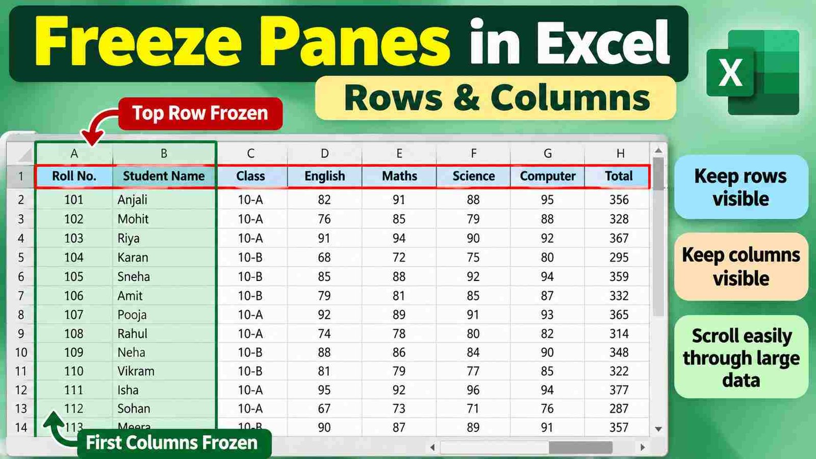
The Freeze Panes feature keeps selected rows or columns visible while you scroll through the rest of a worksheet. For example, you can keep the top heading row on screen while moving down through a long student list. You can also freeze the first column, freeze several rows and columns together, or remove the frozen area whenever it is no longer needed.

The good news is that freezing panes does not require formulas, VBA, or advanced Excel knowledge. It is a simple viewing feature that can make large spreadsheets much easier to read and work with.

In this guide, you will learn how to freeze panes in Excel step by step, how to freeze rows and columns together, how to freeze more than one row, how to unfreeze panes, and how to avoid the common mistakes beginners make.

Visit More:-

1. MS Word Tutorial
2. MS Excel Tutorial
3. MS PowerPoint Tutorial
4. MS Paint Tutorial
5. MS word Formatting Guide: Complete Guide to Format Word Documents

What Is Freeze Panes in Excel?

Freeze Panes in Excel is a worksheet viewing feature that keeps selected rows or columns visible while you scroll through other parts of the worksheet. The frozen area remains on screen, while the unfrozen portion of the spreadsheet can continue moving.

Imagine a worksheet containing 2,000 student records. The headings might be in row 1:

Roll No.	Student Name	Class	Subject	Marks
101	Rahul	10	Mathematics	86
102	Priya	10	Mathematics	91
103	Aman	10	Mathematics	78

When you scroll down to row 700, row 1 normally disappears from the screen. You then have to scroll back to the top to remember what each column means.

By freezing row 1, the headings stay visible while you scroll. This makes the worksheet much easier to understand.

The same idea applies to columns. If the first column contains employee names and you need to scroll horizontally to view many other columns, freezing the first column keeps those names visible.

Why Is Freeze Panes Important?

Freeze Panes is especially helpful when working with large or wide spreadsheets. It reduces the need to repeatedly move back to the top or left side of a worksheet just to identify the information you are looking at.

For students, teachers, office employees, data-entry operators, accountants, and anyone working with Excel regularly, this small feature can save a lot of unnecessary scrolling.

Here are some practical situations where it helps:

• Keeping column headings visible in attendance sheets
• Keeping student names visible while checking marks
• Keeping employee names visible in salary sheets
• Keeping product names visible in inventory records
• Keeping dates visible in monthly reports
• Keeping categories visible in large data tables
• Comparing information across many columns
• Working with lengthy government, business, or academic datasets

A useful way to think about Freeze Panes is this: you are telling Excel which part of the worksheet should stay in place while the rest of the sheet moves.

Freeze Panes in Excel: Quick Overview

Before going into the detailed steps, the main options can be summarized as follows:

Option	What It Does
Freeze Top Row	Keeps the first row visible while scrolling vertically
Freeze First Column	Keeps the first column visible while scrolling horizontally
Freeze Panes	Keeps selected rows, columns, or both visible
Unfreeze Panes	Removes the frozen rows and columns

The Freeze Panes command is more flexible than the first two options because it allows you to select exactly how many rows and columns should remain visible.

How to Freeze the Top Row in Excel

The simplest use of Freeze Panes is keeping the top row visible.

This is useful when the first row contains column headings such as Name, Roll Number, Date, Marks, Department, Salary, or Amount.

Step-by-step method

1. Open your Excel worksheet.
2. Click the View tab on the Ribbon.
3. Find the Freeze Panes option.
4. Click Freeze Panes.
5. Select Freeze Top Row.

That is all you need to do.

Now, when you scroll down the worksheet, the first row will remain visible.

Example

Suppose your worksheet starts like this:

Date	Employee	Department	Attendance	Remarks
01 Sep	Amit	Sales	Present	On Time
01 Sep	Neha	HR	Present	On Time
01 Sep	Ravi	IT	Absent	Leave

After selecting Freeze Top Row, row 1 stays visible as you move down the worksheet.

This is one of the easiest and most useful Excel features for large lists.

How to Freeze the First Column in Excel

Sometimes the important information is arranged horizontally across many columns. In that situation, the first column can disappear when you scroll to the right.

Excel allows you to keep the first column visible.

Step-by-step method

1. Open the worksheet.
2. Go to the View tab.
3. Click Freeze Panes.
4. Select Freeze First Column.

Now column A will remain visible as you scroll horizontally.

Example

Imagine an inventory worksheet:

Product	Jan	Feb	Mar	Apr	May	Jun
Laptop	15	18	21	17	25	29
Monitor	20	22	19	24	27	31
Keyboard	45	41	48	52	55	58

If you need to scroll to the right to see later months, the Product column could move out of view.

Freezing the first column allows you to keep the product names visible while reviewing the monthly data.

How to Freeze Multiple Rows in Excel

You are not limited to freezing only the top row.

Suppose your worksheet has three important rows at the top:

• Row 1: Company or report title
• Row 2: Reporting period
• Row 3: Column headings

You may want all three rows to remain visible.

For this situation, use the main Freeze Panes command rather than Freeze Top Row.

Step-by-step method

Suppose you want to freeze rows 1 to 3.

1. Click the cell in row 4.
2. Go to the View tab.
3. Click Freeze Panes.
4. Select Freeze Panes.

Excel will freeze the rows above the selected cell.

The key idea is simple:

To freeze several rows, select a cell immediately below the last row you want to freeze.

Example

To freeze:

• Rows 1–2 → select A3
• Rows 1–3 → select A4
• Rows 1–5 → select A6
• Rows 1–10 → select A11

The selected row itself does not become frozen. Excel freezes the rows above it.

How to Freeze Multiple Columns in Excel

The same principle works for columns.

Suppose you have a worksheet where columns A and B contain important identifying information. You want both columns to stay visible while scrolling toward the right.

Step-by-step method

To freeze columns A and B:

1. Click a cell in column C.
2. Go to View.
3. Select Freeze Panes.
4. Click Freeze Panes again.

Columns A and B will remain visible.

The important rule is:

To freeze multiple columns, select a cell immediately to the right of the last column you want to freeze.

Examples

Columns to Freeze	Select a Cell In
A	B
A–B	C
A–C	D
A–D	E
A–F	G

This is one of the most important ideas to remember when learning Freeze Panes.

How to Freeze Rows and Columns at the Same Time

This is where Freeze Panes becomes especially useful.

You can freeze both rows and columns together. For example, you might want to keep:

• Rows 1–2 visible at the top
• Columns A–B visible on the left

This is common in large reports where headings are at the top and names or IDs are on the left.

Step-by-step example

Suppose you want to freeze:

• Rows 1 through 3
• Columns A and B

You should select cell C4.

Why C4?

Because:

• Rows above C4 are rows 1, 2, and 3.
• Columns to the left of C4 are columns A and B.

Then:

1. Click cell C4.
2. Open the View tab.
3. Click Freeze Panes.
4. Select Freeze Panes.

Now both the selected rows and columns remain visible while you scroll.

The simple rule

Remember this formula:

Select the cell below the rows and to the right of the columns you want to freeze.

For example:

Want to Freeze	Select
Row 1	A2
Rows 1–2	A3
Column A	B1
Columns A–B	C1
Row 1 + Column A	B2
Rows 1–3 + Columns A–B	C4
Rows 1–5 + Columns A–D	E6

Once you understand this rule, you can freeze almost any combination of top rows and left-side columns.

A Practical Example of Freezing Rows and Columns

Consider a student marksheet with the following structure:

Roll No.	Student Name	Class	English	Maths	Science	Computer	Total	Percentage
101	Anjali	10-A	82	91	88	95	356	89.0%
102	Mohit	10-A	76	85	79	88	328	82.0%
103	Riya	10-A	91	94	90	92	367	91.75%

Now imagine that the file has several additional subjects and hundreds of students.

You may want:

• Row 1 frozen so the subject names remain visible.
• Column A frozen so the roll number remains visible.
• Column B frozen so the student’s name remains visible.

In that situation, select C2 and choose Freeze Panes.

Now you can scroll vertically and horizontally while still seeing the identifying information.

This is much more practical than repeatedly scrolling back to the top or left side.

How to Unfreeze Panes in Excel

Sometimes you freeze a row or column and later decide that you no longer need it.

You do not have to manually undo the effect by scrolling. Excel provides an Unfreeze Panes option.

Step-by-step method

1. Open the View tab.
2. Click Freeze Panes.
3. Select Unfreeze Panes.

The frozen rows and columns will return to normal scrolling behavior.

This is particularly helpful when you are preparing a worksheet for someone else and want to change the viewing arrangement.

Freeze Panes vs Freeze Top Row vs Freeze First Column

These options sound similar, but they are designed for different purposes.

Feature	Best Use
Freeze Top Row	When only the first row contains important headings
Freeze First Column	When only the first column contains important identifying information
Freeze Panes	When you need custom control over rows, columns, or both
Unfreeze Panes	When you want to remove the frozen area

For a simple table, Freeze Top Row may be enough.

For a more complex worksheet, Freeze Panes gives you greater control.

What Happens When You Scroll After Freezing Panes?

When you freeze panes, Excel creates a fixed viewing area.

The frozen rows remain at the top while the lower rows move.

Likewise, frozen columns remain on the left while the other columns move horizontally.

This means your worksheet effectively has two parts:

1. A fixed area that remains visible.
2. A scrolling area that moves as you navigate.

This feature affects how you view the worksheet. It does not change the values in your cells.

For example, if A1 contains “Student Name,” freezing the first row does not move, duplicate, or modify the cell. It simply tells Excel to keep that row visible during scrolling.

Does Freeze Panes Lock the Cells?

No. Freeze Panes and cell protection are different features.

This is a common beginner misunderstanding.

Freeze Panes controls what stays visible when you scroll. It does not prevent someone from changing a cell.

For example, if you freeze row 1, users can still edit cells in row 1 unless some separate protection setting prevents editing.

If your goal is to stop users from changing formulas or values, you need Excel’s protection features instead.

Think of the difference this way:

Feature	Purpose
Freeze Panes	Keep rows/columns visible while scrolling
Protect Sheet	Restrict editing and certain worksheet actions
Hide Rows/Columns	Temporarily hide information from view
Split	Create separate scrolling sections within a worksheet

Knowing the difference can prevent confusion when working with larger spreadsheets.

Freeze Panes vs Split: What Is the Difference?

Freeze Panes and Split may look related because both can divide the worksheet visually, but they serve different purposes.

Freeze Panes keeps a selected top or left section fixed while the rest of the worksheet scrolls.

Split divides the worksheet into separate panes that can be scrolled independently.

For example, if you want row 1 to remain visible while reviewing row 800, Freeze Panes is usually the more natural choice.

If you need to view two distant parts of a worksheet at the same time, the Split feature can sometimes be more appropriate.

The important point is that these features solve different viewing problems.

How to Know Which Cell to Select Before Using Freeze Panes

This is probably the most important skill to understand.

Many beginners click the wrong cell and then wonder why the wrong rows or columns were frozen.

Use this simple method:

To freeze rows

Select the row immediately below the last row you want frozen.

To freeze columns

Select the column immediately to the right of the last column you want frozen.

To freeze rows and columns

Select the cell that is:

• Below the last row you want frozen, and
• To the right of the last column you want frozen.

Example

Suppose you want to freeze:

• Rows 1–4
• Columns A–C

The correct cell is D5.

Why?

• Rows 1–4 are above row 5.
• Columns A–C are to the left of column D.

Then choose View → Freeze Panes → Freeze Panes.

This rule works across many spreadsheet layouts.

Common Mistakes When Freezing Panes

Learning the feature is easy, but a few mistakes are very common.

Selecting the wrong cell

This is the most frequent problem.

Suppose you want to freeze rows 1–3 but select A3 instead of A4. Excel freezes only the rows above the selected cell.

Remember:

The selected row is not part of the frozen area.

Choosing Freeze Top Row when several rows are needed

Freeze Top Row only affects the first row.

If you need rows 1–3 or rows 1–5, select the correct cell and use the main Freeze Panes command.

Choosing Freeze First Column when several columns are needed

Freeze First Column affects only column A.

For multiple columns, select the first column outside the frozen area.

Freezing unnecessary information

Freezing too many rows or columns can reduce your available workspace.

Suppose you freeze the first eight rows even though only row 1 contains useful headings. A significant portion of the screen may remain occupied by information that you do not need while scrolling.

Freeze only what helps you identify the data.

Confusing freezing with protecting

Freezing a worksheet area does not prevent editing. These are separate Excel features.

Forgetting to unfreeze old settings

Sometimes you try to create a new freeze arrangement while an existing one is still active.

If the behavior does not match what you expect, check the View → Freeze Panes menu and use Unfreeze Panes first. Then apply the new setup.

How Freeze Panes Helps Students

Students often use Excel for attendance records, marksheets, project data, survey results, timetables, and practical assignments.

Freeze Panes can make these files much easier to navigate.

For example, a student may create a worksheet with:

• Student Name
• Roll Number
• English
• Mathematics
• Science
• Social Science
• Computer
• Total
• Percentage
• Grade

Once the number of rows becomes large, the headings can disappear while scrolling.

Freezing the top row keeps the subject names visible.

This also makes it easier to understand data while preparing assignments and presentations.

Practical study tip

When working on an Excel assignment involving a large table, ask yourself:

“Which information do I need to see all the time to understand the numbers below?”

That information is usually a good candidate for freezing.

Freeze Panes for Competitive Exam and Job-Related Work

Excel is often used for lists of applicants, attendance data, marks, schedules, document tracking, and reporting.

For example, imagine an application-tracking sheet containing:

Application ID	Candidate Name	Category	Post	Exam Date	Status	Documents	Remarks

If the file contains a large number of candidates, scrolling down can make it difficult to remember which column represents which detail.

Freezing the top row helps keep the headings visible.

If Application ID and Candidate Name are in the first two columns, freezing those columns can also make the sheet easier to review while scrolling horizontally.

The same principle can be useful for teachers, office staff, recruitment teams, school administrators, and people maintaining records.

Freeze Panes in Excel for Large Data Tables

Large data tables become easier to work with when the structure remains visible.

Consider a financial worksheet containing columns such as:

• Date
• Transaction ID
• Customer
• Category
• Amount
• Tax
• Payment Method
• Status
• Remarks

With hundreds or thousands of transactions, the headings quickly disappear during vertical scrolling.

Freezing the heading row provides a constant reference point.

The feature becomes even more useful when a worksheet contains both many rows and many columns.

For example, you might freeze the first one or two rows as headings and freeze a key identifier column on the left.

Freeze Panes in Wide Worksheets

A worksheet can be difficult to navigate horizontally when it contains dozens of columns.

For instance, a monthly report could contain separate columns for:

• January
• February
• March
• April
• May
• June
• July
• August
• September
• October
• November
• December

It may also have columns for multiple categories or departments.

When you scroll right, the original identifying columns may disappear.

Freezing the necessary left-side columns helps maintain context.

This is especially useful when comparing values across distant columns.

Does Freeze Panes Work With Formulas?

Yes. Freeze Panes is independent of formulas.

You can freeze a worksheet containing:

• SUM formulas
• AVERAGE formulas
• IF formulas
• VLOOKUP formulas
• XLOOKUP formulas
• COUNTIF formulas
• Percentage calculations
• Dates
• Text data

Freezing panes does not change the formulas themselves.

For example, if a Total column contains a SUM formula, freezing the header row will not alter that calculation.

The feature changes the viewing behavior, not the underlying data.

Does Freeze Panes Affect Printing?

Freeze Panes is primarily a screen-viewing feature.

This distinction is important.

A row that is frozen for scrolling is not automatically the same as a row that repeats on every printed page.

If your goal is to repeat headings when printing a worksheet across multiple pages, Excel provides separate page setup options for repeating rows or columns during printing.

So, when preparing a report, distinguish between:

Freeze Panes for on-screen navigation and print-title settings for printed pages.

They solve different problems.

Best Practices for Using Freeze Panes

Freeze Panes is most useful when you apply it thoughtfully.

Freeze only the information you need

Do not freeze large areas simply because Excel allows it.

A compact frozen area generally leaves more room for the actual data.

Keep important identifiers visible

Names, IDs, dates, or categories are often more useful to freeze than decorative title rows.

Use Freeze Top Row for simple tables

If your table has only one heading row, the built-in Freeze Top Row option is quick and clear.

Use custom Freeze Panes for complex reports

When a report contains multiple heading rows or important left-side identifiers, custom Freeze Panes is usually more flexible.

Check the result after applying it

Scroll vertically and horizontally after freezing to make sure the correct information stays visible.

Unfreeze before changing the layout

If an existing freeze setting becomes confusing, unfreeze it and create a new arrangement from scratch.

This is often easier than trying to work around the old setting.

How to Use Freeze Panes Efficiently on Mobile or Different Excel Versions

Excel is available across different platforms, including desktop applications and web-based environments. The exact Ribbon arrangement and interface can change between versions.

The general concept remains the same, but menu names or locations may look slightly different depending on the version you use.

On a Windows desktop version of Excel, the View tab commonly contains the Freeze Panes command.

When working in Excel for the web or another edition, check the current View-related commands if the interface looks different.

The underlying principle remains:

• Select the correct cell.
• Use the Freeze Panes command.
• Define the area that should remain visible.

How to Freeze the First Two Rows and First Column

Let us take a slightly more advanced example.

Suppose a worksheet has:

• Row 1: Report title
• Row 2: Column headings
• Column A: Serial Number

You want rows 1–2 and column A to stay visible.

The correct cell is B3.

Then:

1. Select B3.
2. Open View.
3. Select Freeze Panes.
4. Choose Freeze Panes.

Now:

• Rows 1 and 2 stay at the top.
• Column A stays on the left.

This is a useful arrangement for reports where both the heading area and a key identifier need to remain visible.

How to Freeze the First Three Rows and First Two Columns

Suppose your worksheet contains:

• Rows 1–3 as heading information
• Columns A–B as identification information

You want all of these sections visible while scrolling.

The correct cell is C4.

Why?

Rows 1–3 are above C4, and columns A–B are to the left of C4.

Then:

View → Freeze Panes → Freeze Panes

This freezes the desired area.

A useful mental picture is:

Frozen Rows	Frozen Columns	Starting Cell
1	A	B2
1–2	A	B3
1–3	A–B	C4
1–5	A–C	D6

Once you understand this pattern, the feature becomes much easier.

How to Fix a Freeze Panes Setting That Looks Wrong

Sometimes users think Excel is malfunctioning when the wrong rows or columns remain fixed.

Usually, the problem is simply that the incorrect starting cell was selected.

Try this process:

1. Go to View.
2. Select Freeze Panes.
3. Click Unfreeze Panes.
4. Click the correct cell.
5. Open Freeze Panes again.
6. Select Freeze Panes.

For example, if you want rows 1–4 and columns A–B frozen, select C5, not C4 or B5.

This reset-and-apply method is easy to remember and useful when troubleshooting.

Important Points to Remember

Here are the main rules worth memorizing:

1. Freeze Top Row keeps only row 1 visible.
2. Freeze First Column keeps only column A visible.
3. To freeze multiple rows, select a cell below those rows.
4. To freeze multiple columns, select a cell to the right of those columns.
5. To freeze rows and columns together, select a cell below and to the right of the area you want to freeze.
6. Use Unfreeze Panes to remove the current frozen area.
7. Freeze Panes changes screen navigation, not the underlying cell values.
8. Freeze Panes is different from worksheet protection.
9. Freezing too many rows or columns can reduce the visible workspace.
10. The exact menu layout may differ between Excel versions.

A Simple Memory Trick for Freeze Panes

A helpful shortcut for remembering how the feature works is:

“Freeze everything above and to the left.”

When you choose a cell and apply Freeze Panes:

• Everything above the selected cell can be frozen.
• Everything to the left of the selected cell can be frozen.

The selected cell itself marks the beginning of the scrolling area.

For example:

If you select D6, Excel can freeze:

• Rows 1–5
• Columns A–C

This single rule makes custom Freeze Panes much easier to understand.

Common Questions About Freeze Panes

What is Freeze Panes in Excel?

Freeze Panes in Excel keeps selected rows or columns visible while you scroll through the rest of the worksheet. It is mainly used to keep headings or identifying information visible when working with large spreadsheets.

How do I freeze the top row in Excel?

Go to View → Freeze Panes → Freeze Top Row. The first row will remain visible while you scroll vertically through the worksheet.

How do I freeze the first column in Excel?

Go to View → Freeze Panes → Freeze First Column. Column A will remain visible while you scroll horizontally.

How do I freeze multiple rows in Excel?

Select the cell immediately below the last row you want to freeze. Then choose View → Freeze Panes → Freeze Panes.

For example, to freeze rows 1–4, select a cell in row 5.

How do I freeze multiple columns in Excel?

Select the cell immediately to the right of the last column you want to freeze. Then choose View → Freeze Panes → Freeze Panes.

For example, to freeze columns A–C, select a cell in column D.

How do I freeze rows and columns together?

Select the cell below the rows and to the right of the columns you want to freeze. Then go to View → Freeze Panes → Freeze Panes.

For example, select C4 to freeze rows 1–3 and columns A–B.

How do I unfreeze panes in Excel?

Go to View → Freeze Panes → Unfreeze Panes. This removes the current frozen rows and columns.

Does Freeze Panes lock cells from editing?

No. Freeze Panes controls scrolling and visibility. It does not prevent users from editing cells. To restrict editing, you need worksheet or workbook protection features.

Can I freeze both a row and a column in Excel?

Yes. You can freeze both at the same time by selecting the appropriate cell before choosing Freeze Panes.

For example, selecting B2 allows the first row and first column to remain visible.

Why is Excel freezing the wrong row or column?

The usual reason is that the wrong cell was selected before applying Freeze Panes. Remember that Excel freezes the rows above and columns to the left of the selected cell.

Can I freeze more than one row and more than one column?

Yes. Excel allows you to create a custom frozen area. Select the cell that is below the rows and to the right of the columns you want to keep visible.

Practical Exercises to Learn Freeze Panes

The best way to understand this feature is to try a few simple exercises.

Exercise 1: Freeze the top row

Create a table with 50 or more rows.

Add headings in row 1.

Then:

View → Freeze Panes → Freeze Top Row

Scroll downward and observe the heading.

Exercise 2: Freeze two rows

Put a title in row 1 and headings in row 2.

Select A3 and use Freeze Panes.

Scroll down and check whether both rows remain visible.

Exercise 3: Freeze two columns

Enter names in column A and IDs in column B. Add several additional columns to the right.

Select C1 and apply Freeze Panes.

Scroll horizontally to confirm that columns A and B stay visible.

Exercise 4: Freeze rows and columns together

Create a larger table and use:

• Rows 1–2 for headings
• Columns A–B for identifiers

Select C3 and apply Freeze Panes.

Then scroll both vertically and horizontally.

These exercises help turn the concept from something you have read into something you can confidently use.

When Should You Not Use Freeze Panes?

Freeze Panes is useful, but it does not need to be enabled on every worksheet.

You may not need it when:

• The worksheet contains only a few rows.
• The entire dataset fits comfortably on one screen.
• There are no important headings to keep visible.
• You are working with a small calculation sheet.
• The frozen area would take up too much screen space.

The goal is not to use every Excel feature. The goal is to make the worksheet easier to use.

Final Checklist for Freeze Panes in Excel

Before finishing your worksheet, check these points:

Question	What to Check
Are the headings disappearing?	Freeze the required top row or rows
Are important left-side labels disappearing?	Freeze the required columns
Do you need both?	Select the correct cell and use Freeze Panes
Did you freeze the wrong area?	Unfreeze and apply it again
Is too much of the screen occupied?	Reduce the number of frozen rows or columns
Are you trying to prevent editing?	Use sheet protection instead
Is your Excel version different?	Check the current View menu in your version

Conclusion

Freeze Panes in Excel is one of those simple features that becomes extremely valuable once you start working with larger worksheets. Instead of repeatedly scrolling back to find column headings, names, IDs, or other reference information, you can keep the important area visible while the rest of the worksheet moves.

For basic tables, you can use Freeze Top Row or Freeze First Column. For more advanced layouts, the main Freeze Panes command lets you freeze multiple rows, multiple columns, or both at the same time.

The most useful rule to remember is simple: select the cell below and to the right of the area you want to keep visible, then choose View → Freeze Panes → Freeze Panes.

Once you understand that rule, freezing a worksheet becomes much easier. Whether you are preparing student marks, maintaining attendance, reviewing records, creating reports, or managing a large dataset, this feature can make Excel more comfortable and organized to use.